Margins, Kernels, and Support Vectors: An Intuitive Guide to SVMs

We have seen in previous machine learning models that classification often comes down to finding the right decision boundary. But what makes one boundary better than another? SVMs (Support Vector Machines) answer this question geometrically: an optimal decision boundary is the one that maximizes the distance between the closest points of different classes, allowing us to better distinguish between the two and make better, more confident predictions. This geometric approach makes SVMs an elegant solution to finding an optimal decision boundary and is intuitive to visualize. With the help of kernels, it allows SVMs to handle complex problems that aren’t linearly separable.

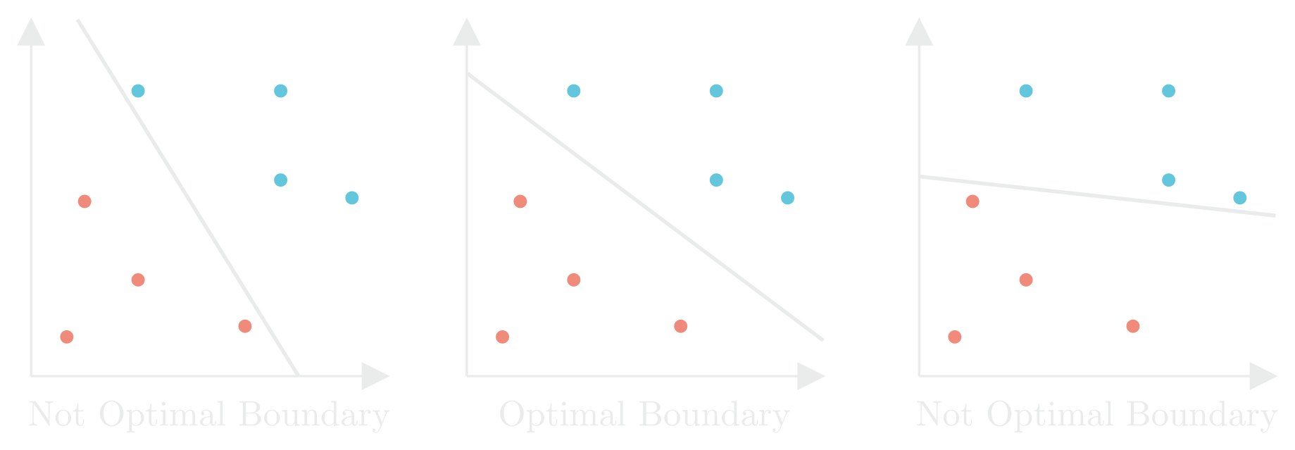
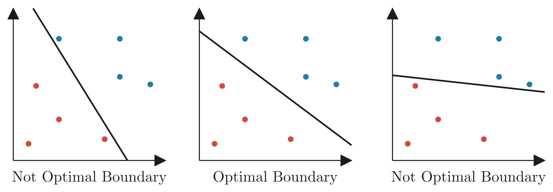
Intuition of Margin

When training a classifier, it’s not enough to simply draw a line that separates the two classes. Like we saw in logistic regression, we also care about how confident we are in our predictions.

• Points far from the decision boundary are classified with high confidence
• Points near the boundary are uncertain, since even a slight shift could flip their predicted label

This distance from an example to the decision boundary is what we call the margin.

Margin Calculation

The margin for training example $x_i$ for a decision boundary defined by $w^Tx_i=0$ is:

$$\gamma_i = \frac{y_i \,(w^T x_i)}{\|w\|}$$

Since the weight vector $w$ is perpendicular to our decision boundary at every possible $x$, when we compute the dot product $w^T x_i$, we’re really asking:

“How far does $x_i$ extend in the direction of the normal vector $w$?”

The sign of this value tells us which side of the boundary the point lies on. However, this raw value isn’t a true distance; it depends on the scale of $w$. If we doubled $w$, every dot product would double as well. To remove this dependence, we normalize by the length of $w$.

Incorporating Labels

The signed distance alone doesn’t account for which class the point should belong to. To fix this, we multiply by the true label $y_i \in \{+1, -1\}$:

• If $x_i$ is correctly classified, $\gamma_i > 0$.
• If $x_i$ is misclassified, $\gamma_i < 0$.

In other words, multiplying by $y_i$ “flips” the sign when needed so that the margin is always positive for correct predictions and negative for incorrect ones.

Margin of the Dataset

For a dataset with $m$ training examples, we care about the smallest margin across all points, since the point closest to the boundary is the most vulnerable to misclassification. Formally:

$$\gamma = \min \{ \gamma_1, \gamma_2, \dots, \gamma_m \}$$

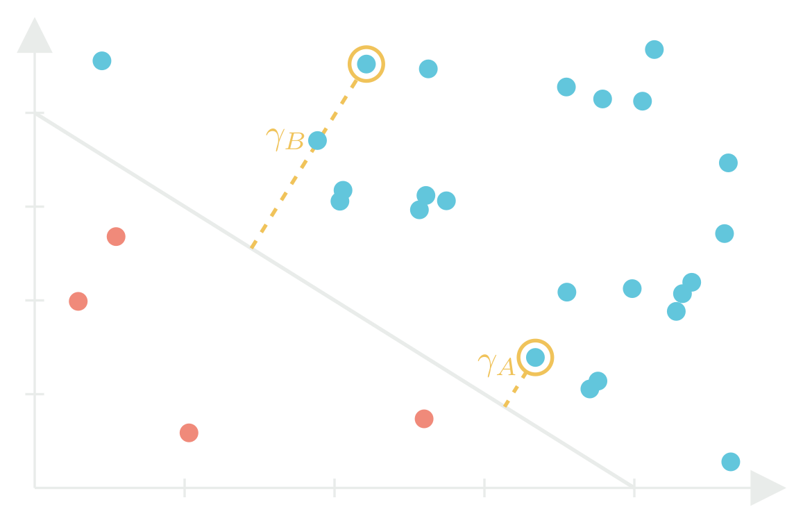
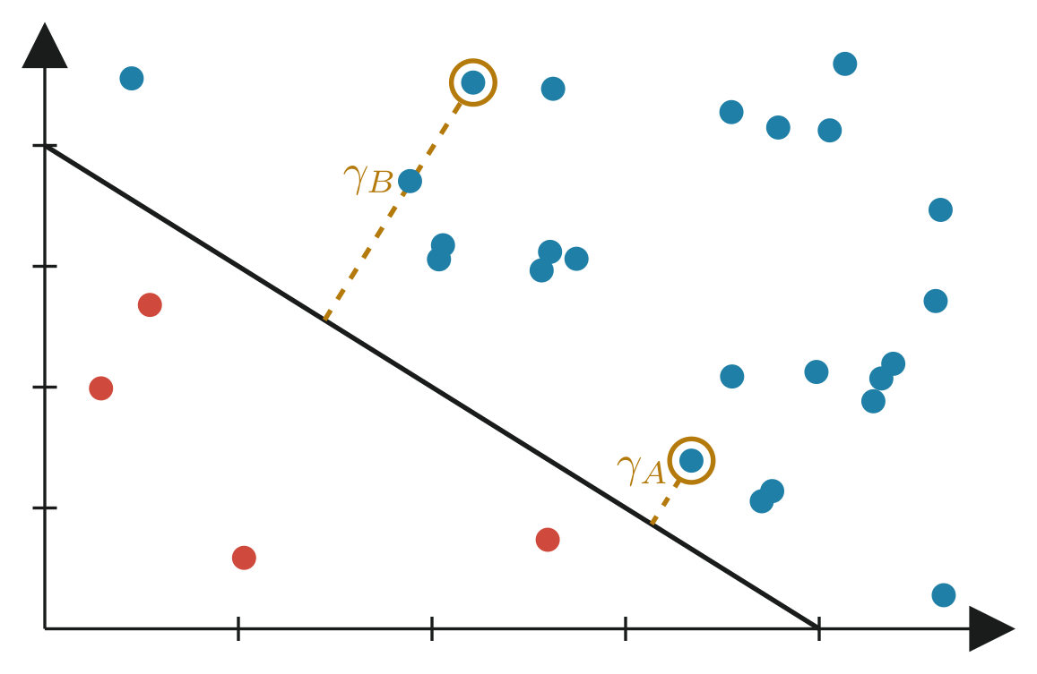
• Point A has a small margin, so we are less confident in its classification.
• Point B has a large margin, so we are more confident in its classification.

Support Vectors

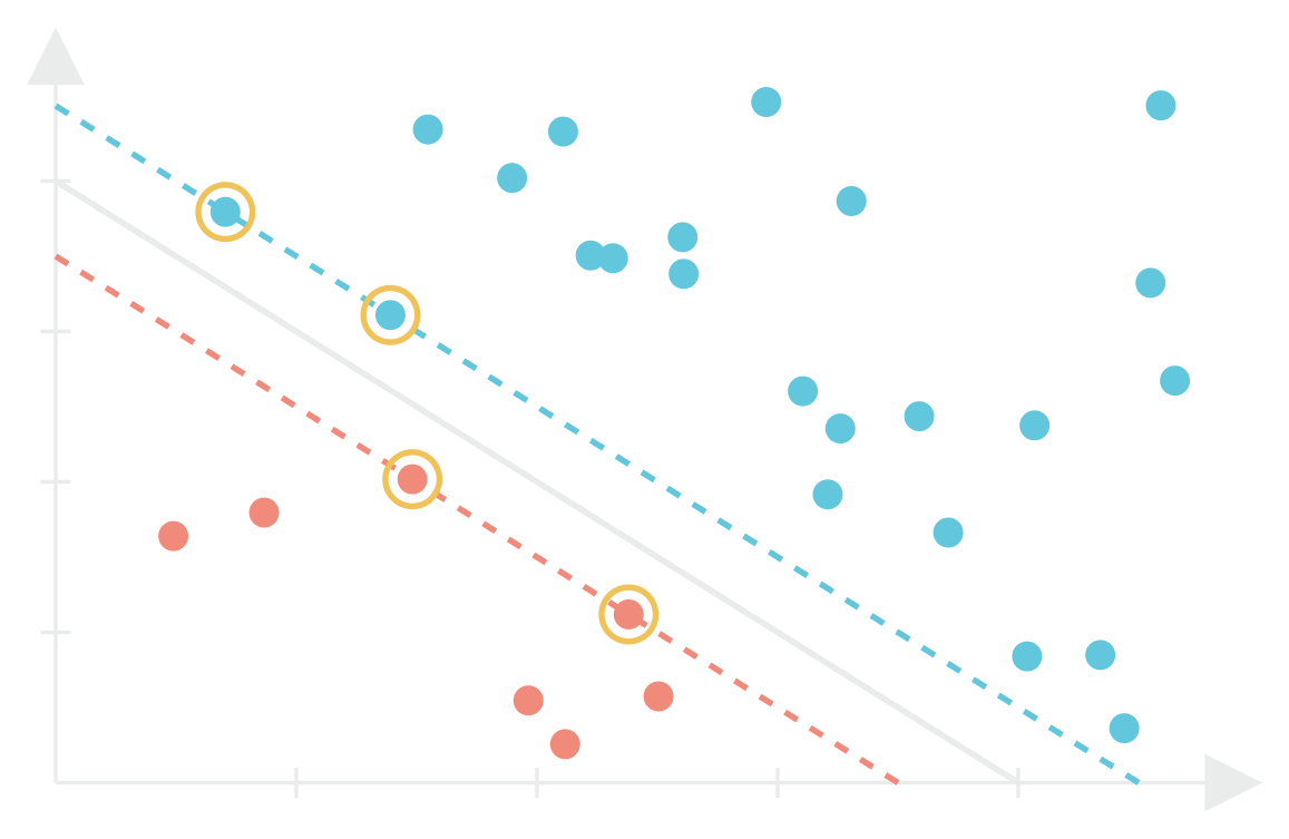
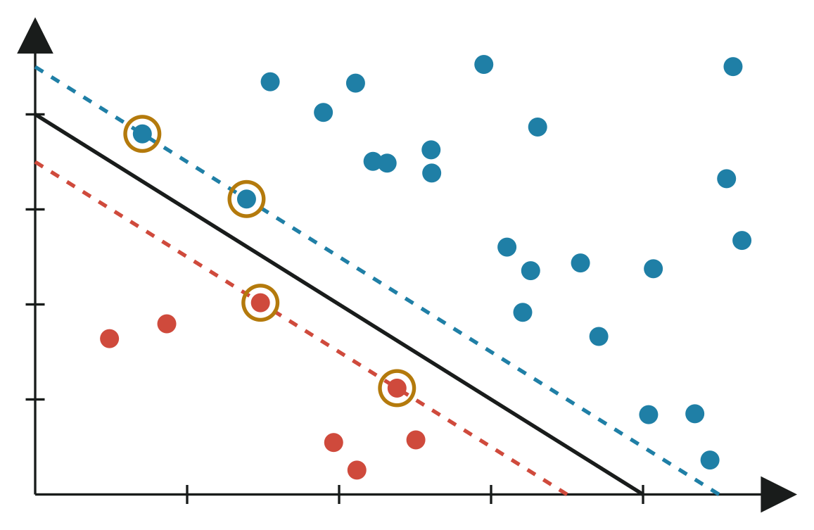
The points from either class that lie closest to the decision boundary are special points called support vectors. These points are critical because:

• They define the margin width.
• If you moved them, the decision boundary would shift.
• If you removed all other points and kept only the support vectors, the SVM would learn the exact same boundary.

From Margins to Optimization

Now that we know what a margin is, the central goal of an SVM becomes clear: we want to maximize the smallest margin across all training examples. This makes the decision boundary between two classes as wide as possible.

Since the smallest margin is determined by the support vectors, the problem boils down to finding the decision boundary that creates the largest possible gap between the closest points of the two classes.

Formally, this can be written as a constrained optimization problem:

$$\underset{w}{\max} \enspace \gamma \enspace \text{subject to} \enspace \frac{y_i (w^Tx_i)}{\|w\|} \geq \gamma, \forall i$$

Each constraint says: for every data point $x_i$, its margin $\frac{y_i(w^Tx_i)}{\|w\|}$ must be at least $\gamma$.

The Primal Problem

Optimizing this directly is tricky because both $\gamma$ and $w$ appear together in the same fraction. Luckily, SVMs can exploit a helpful property: if we scale $w$, the decision boundary doesn’t change; it just rescales the margin. This means that we can fix the scale in a convenient way by requiring the support vectors to satisfy:

$$y_i (w^Tx_i) = 1$$

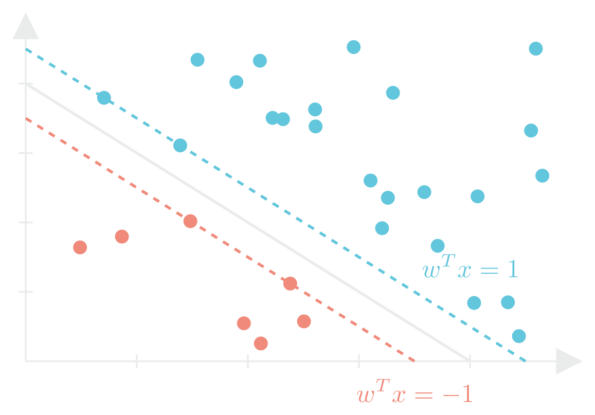
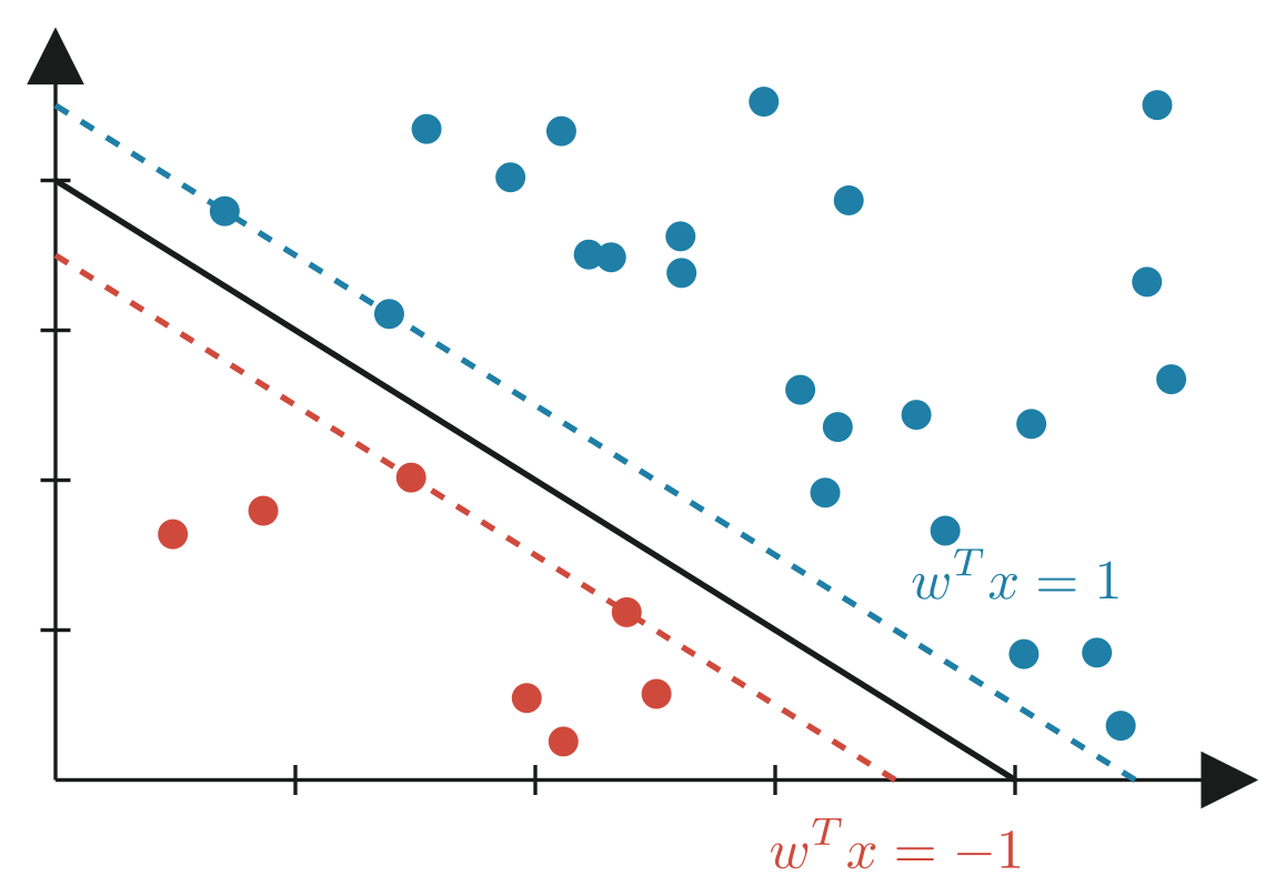
Under this normalization, the margin becomes:

$$\gamma = \frac{1}{\|w\|}$$

So maximizing the margin $\gamma$ is equivalent to minimizing the size of $w$. Our optimization problem becomes:

$$\underset{w}{\min} \; \frac{1}{2} {\|w\|}^2 \enspace \text{subject to} \enspace y_i (w^Tx_i) \geq 1, \enspace \forall i$$

Note: the $\frac{1}{2}$ is just a mathematical convenience — it makes the derivatives cleaner when solving and doesn’t affect the solution.

This is the primal problem: it forces every point to be on the correct side of the boundary, at least 1 unit away.

At this stage, it is not obvious how to actually solve this problem. We need a systematic way to make $w$ as small as possible while still respecting all the margin constraints.

Lagrangian Functional

For constrained optimization, a standard tool is the Lagrangian functional:

$$\mathcal{L}(x, \lambda) = f(x) + \sum_i \lambda_i g_i(x)$$

where:

• $f(x)$ is the objective function we want to minimize,
• $g_i(x)$ are the inequality constraints,
• $\lambda_i \geq 0$ are the Lagrange multipliers.

Intuition

The Lagrangian takes the original objective and adds penalties for violating constraints.

• If $g_i(x) \leq 0$, the constraint is satisfied and the penalty is zero.
• If $g_i(x) > 0$, then the constraint is violated, and $\lambda_i g_i(x)$ makes the objective larger (worse).

Thus, the optimizer naturally avoids constraint violations. This allows us to rewrite the primal problem:

$$\underset{x}{\min} \; f(x) \enspace \text{subject to} \enspace g_i(x) \leq 0, \enspace \forall i \enspace \Longleftrightarrow \enspace \underset{x}{\min} \; \underset{\lambda}{\max} \; \mathcal{L}(x, \lambda)$$

Why the maximization over $\lambda$?

Because some multipliers could otherwise be set to zero, “ignoring” violated constraints. Maximizing over $\lambda$ finds the harshest penalties that make violations impossible to exploit.

The Dual Problem

So far, the order has been maximize $\lambda$, then minimize $x$. That’s the primal problem. But what if we flip the order?

$$\underset{\lambda}{\max} \; \underset{x}{\min} \; \mathcal{L}(x, \lambda)$$

In this case, we find values of $x$ that minimize the objective function first, regardless of whether they violate any constraints. Then we maximize over $\lambda$, trying to push the minimized value up as much as possible.

This is the dual problem.

• It doesn’t guarantee feasibility directly.
• Instead, it produces a lower bound on the primal optimum. This is called weak duality.

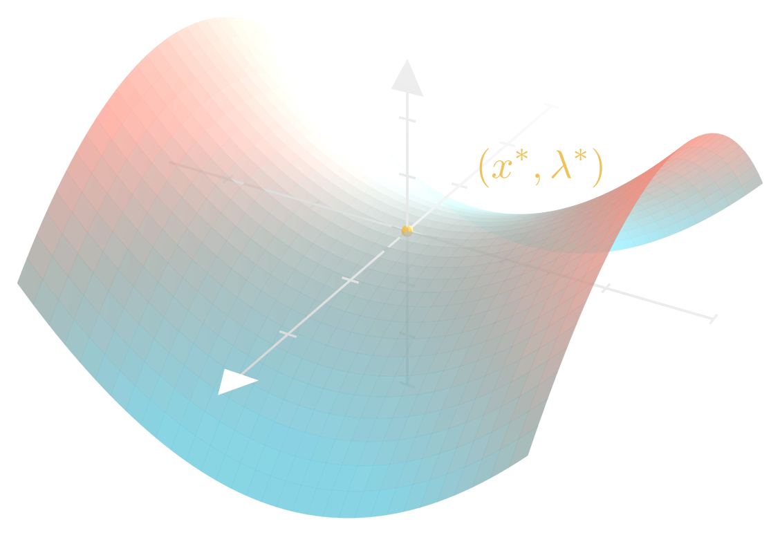
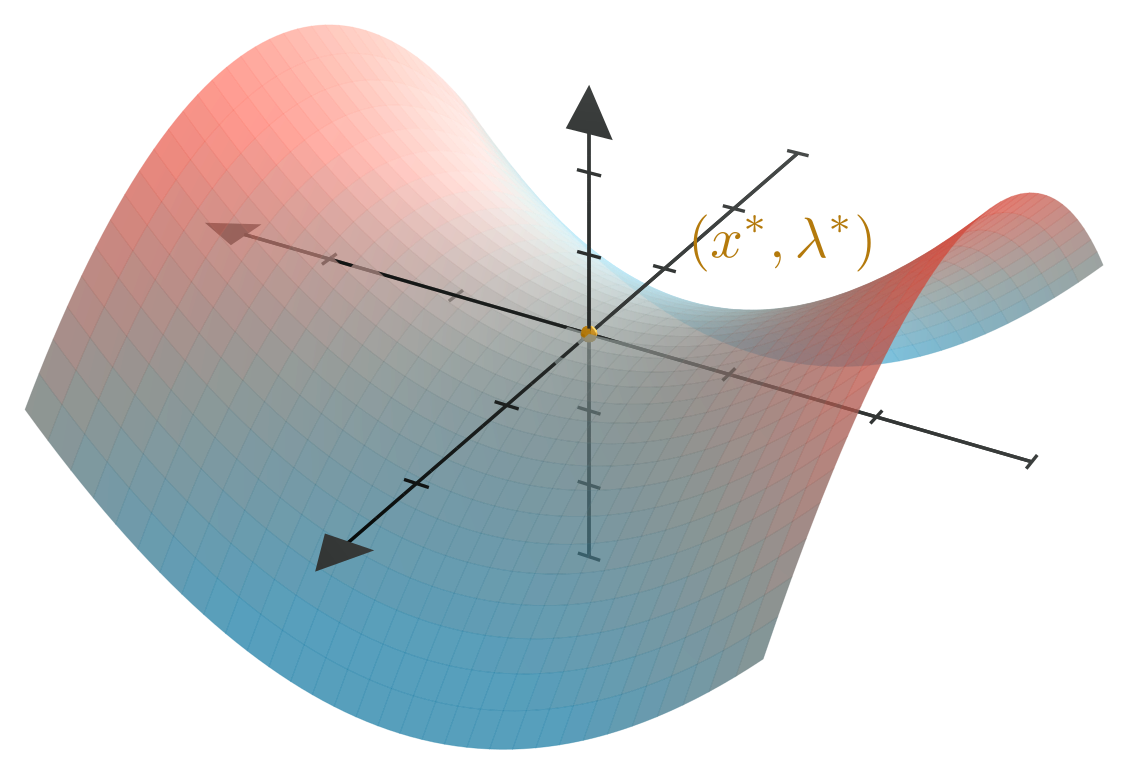
If the optimal values of the primal and dual problems are equal, this is called strong duality. When strong duality holds, the optimal solution is a saddle point of the Lagrangian.

$$\underset{\lambda}{\max} \; \underset{x}{\min} \; \mathcal{L}(x, \lambda) \leq \underset{x}{\min} \; \underset{\lambda}{\max} \; \mathcal{L}(x, \lambda)$$

Finding the Optimal Solution

How do we know when we’ve reached the saddle point? This is where the Karush-Kuhn-Tucker (KKT) conditions come in. They provide the necessary conditions for optimality. The KKT conditions are:

1. Primal feasibility — all constraints are satisfied:

   $$g_i(x^*) \leq 0, \enspace \forall i$$

2. Dual feasibility — all multipliers are nonnegative:

   $$\lambda_i^* \geq 0, \enspace \forall i$$

3. Stationarity — the gradient of the Lagrangian vanishes:

   $$\nabla_x \mathcal{L}(x^*, \lambda^*) = 0$$

4. Complementary slackness — each constraint is either satisfied or ignored:

   $$\lambda_i^* g_i(x^*) = 0, \enspace \forall i$$

   (if a constraint is satisfied, its multiplier can be positive; otherwise, the multiplier must be zero)

Together, these conditions certify that $(x^*, \lambda^*)$ is the optimal solution.

Using the Lagrangian With SVMs

Now that we’ve built some intuition for how the Lagrangian balances the objective function against penalties, we can apply it directly to our SVM optimization problem. The primal SVM objective is:

$$\underset{w}{\min} \; \frac{1}{2} {\|w\|}^2 \enspace \text{subject to} \enspace y_i (w^Tx_i) \geq 1, \enspace \forall i$$

Here:

• The objective function is $f(w) = \frac{1}{2} {\|w\|}^2$

• The constraints can be rewritten as:

$$g_i(w) = y_i (w^Tx_i) \geq 1 \enspace \Rightarrow \enspace 1 - y_i (w^Tx_i) \leq 0$$

The Lagrangian then becomes:

$$\mathcal{L}(w, \lambda) = \frac{1}{2} {\|w\|}^2 + \sum_{i=1}^m \lambda_i \left[ 1 - y_i (w^Tx_i) \right]$$

Step 1. Stationarity

The stationary KKT condition says that at the optimal weights $w^*$, the gradient of the Lagrangian with respect to $w$ vanishes. Since our objective is convex, this stationary point is indeed the minimum.

Important: this condition alone does not guarantee that $w^*$ is feasible. Feasibility comes from the other KKT conditions.

Taking the gradient:

$$\begin{align*} \nabla_w \mathcal{L}(w, \lambda) &= w + \sum_{i=1}^m \lambda_i \left(- y_i x_i \right) = 0\\ &\Downarrow\\ w^* &= \sum_{i=1}^m \lambda_i y_i x_i \end{align*}$$

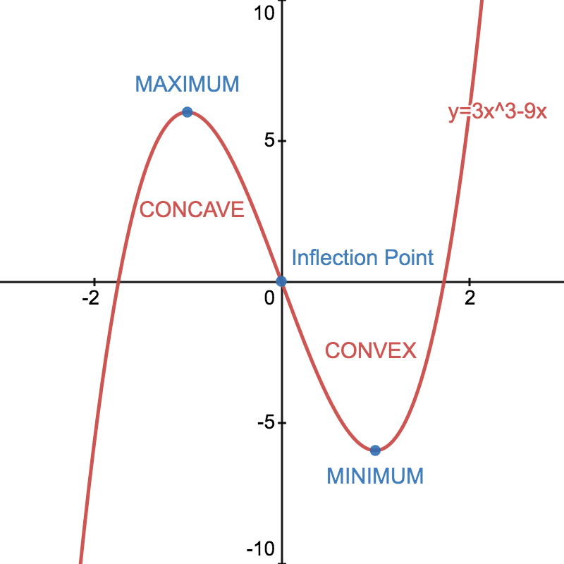
Notice that only the training points where $\lambda_i > 0$ contribute to $w^*$. These points are our support vectors!

Step 2. Substituting Back into Lagrangian

We now plug $w^*$ into the Lagrangian to eliminate $w$:

$$\mathcal{L}(w^*, \lambda) = \frac{1}{2} {\|w^*\|}^2 + \sum_{i=1}^m \lambda_i \left[ 1 - y_i (w^{*T}x_i) \right]$$

After simplification, this becomes:

$$\sum_{i=1}^m \lambda_i - \frac{1}{2} \sum_{i=1}^m \sum_{j=1}^m \lambda_i \lambda_j y_i y_j x_i^T x_j$$

$\|w^*\|^2 = w^{*T}w^* = \Big(\sum_i \lambda_i y_i x_i\Big)^T \Big(\sum_j \lambda_j y_j x_j\Big) = \sum_i \sum_j \lambda_i \lambda_j y_i y_j x_i^T x_j$

Step 3. The Dual Problem

Because we’ve already minimized over $w$, what remains is to maximize over $\lambda$. This gives us the dual problem:

$$\underset{\lambda}{\max} \sum_{i=1}^m \lambda_i - \frac{1}{2} \sum_{i=1}^m \sum_{j=1}^m \lambda_i \lambda_j y_i y_j x_i^T x_j \enspace \text{subject to} \enspace \lambda_i \geq 0, \enspace \forall i$$

Here, we’ve explicitly enforced the dual feasibility KKT condition. The other KKT conditions, primal feasibility and complementary slackness, are guaranteed to hold at the optimal solution (thanks to convexity and strong duality).

This dual is a quadratic programming (QP) problem. In practice, it can be solved efficiently using the SMO algorithm.

Step 4. Recovering the Weights

Once we solve for the optimal multipliers $\lambda^*$, we can recover the optimal weights to get our decision boundary:

$$w^* = \sum_{i=1}^m \lambda_i^* y_i x_i$$

Soft-Margin SVMs

So far, we’ve assumed the data is perfectly linearly separable. In practice, this almost never happens. Real datasets are noisy, overlapping, or mislabeled. If we insisted on perfect separation, the SVM could overfit badly or even fail to find a solution.

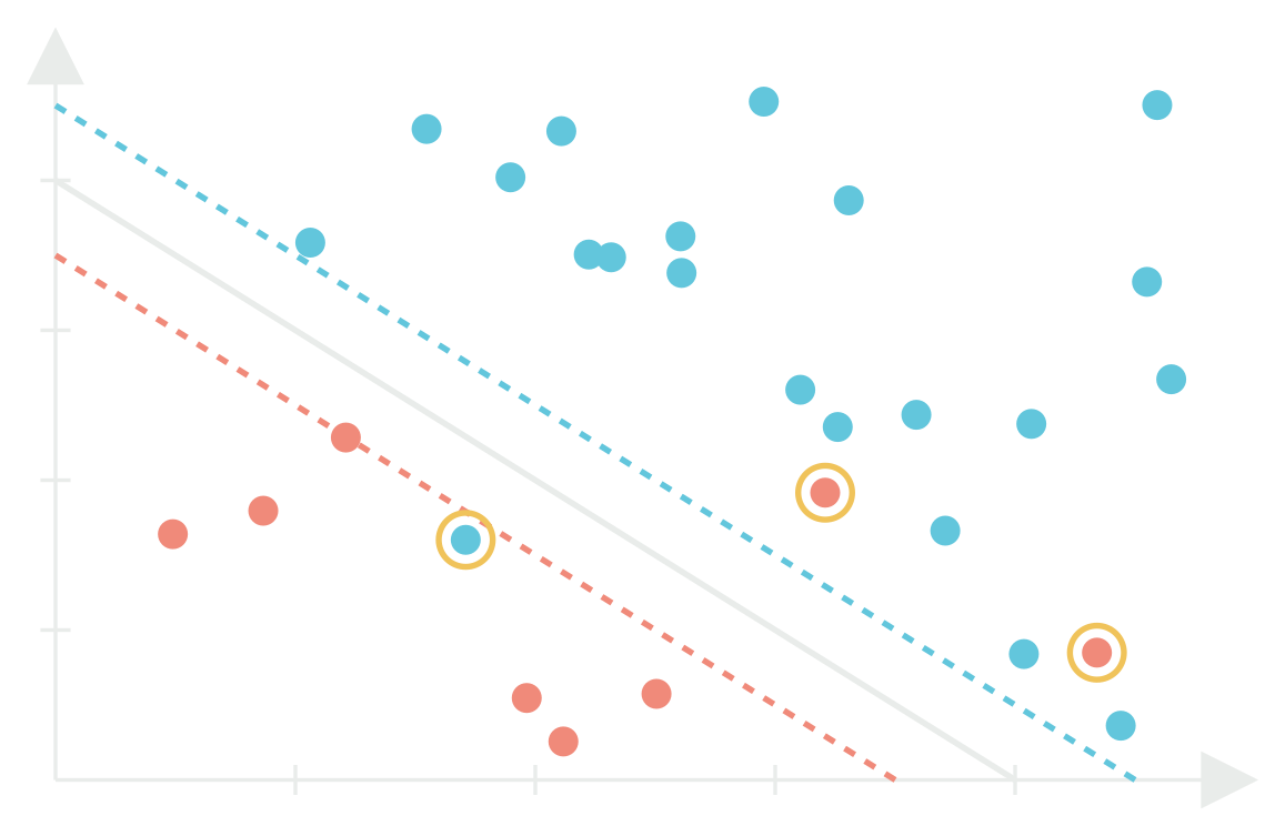
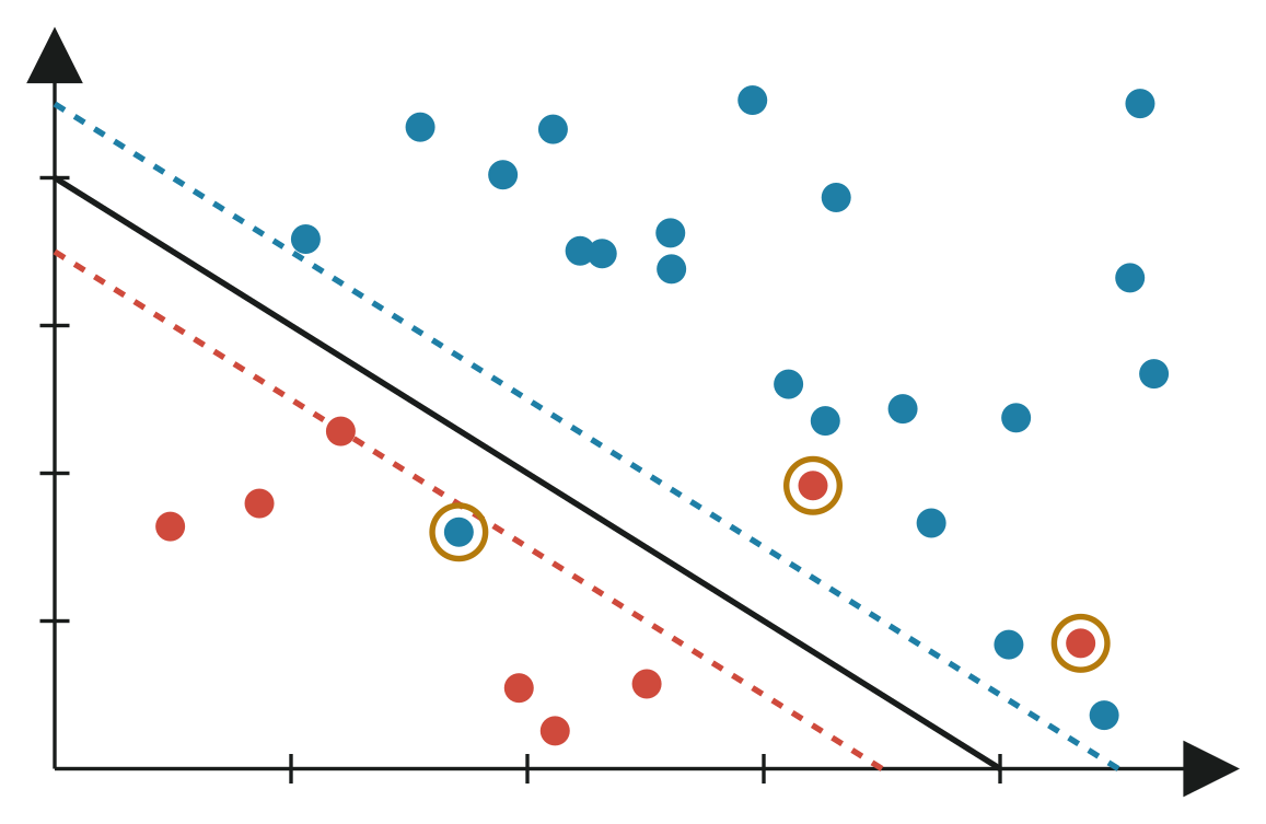
To handle this, SVMs introduce soft margins. Instead of requiring every point to lie strictly outside the margin, we allow some points to be inside or even misclassified, but we penalize these violations.

Slack Variables

We introduce a nonnegative slack variable $\xi_i \geq 0$ for each training point:

$$y_i (w^T x_i) \geq 1 - \xi_i$$

• If $\xi_i = 0$, the point is correctly classified and outside the margin.
• If $0 < \xi_i < 1$, the point is inside the margin but still on the correct side.
• If $\xi_i > 1$, the point is misclassified.

The Soft-Margin Objective

Our optimization problem becomes:

$$\min_{w, \xi} \;\; \tfrac{1}{2}\|w\|^2 + C \sum_{i=1}^m \xi_i \enspace \text{subject to} \enspace y_i (w^T x_i) \geq 1 - \xi_i, \enspace \xi_i \geq 0, \enspace \forall i$$

Here, $C > 0$ is a hyperparameter that controls the trade-off:

• Large $C$: fewer violations (stricter fit, risk of overfitting).
• Small $C$: more violations allowed (looser fit, better generalization).

Kernel Functions

With soft margins, SVMs can handle noisy or overlapping data: instead of requiring perfect separation, they balance margin width against some classification errors.

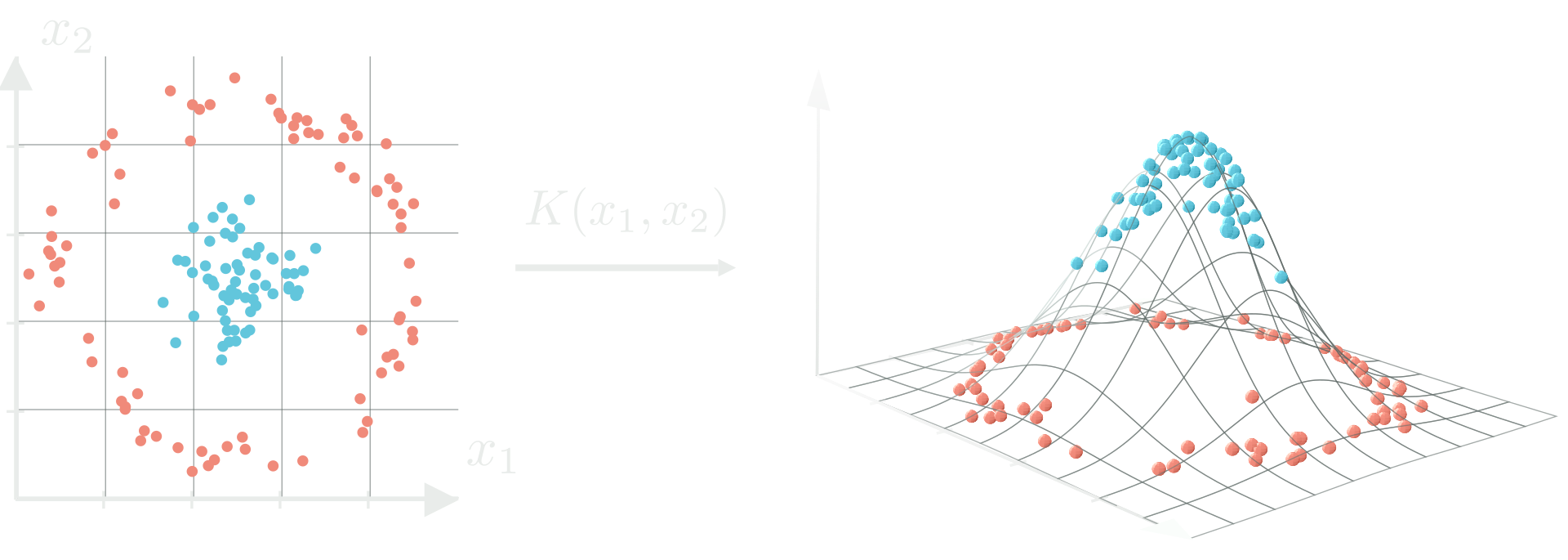
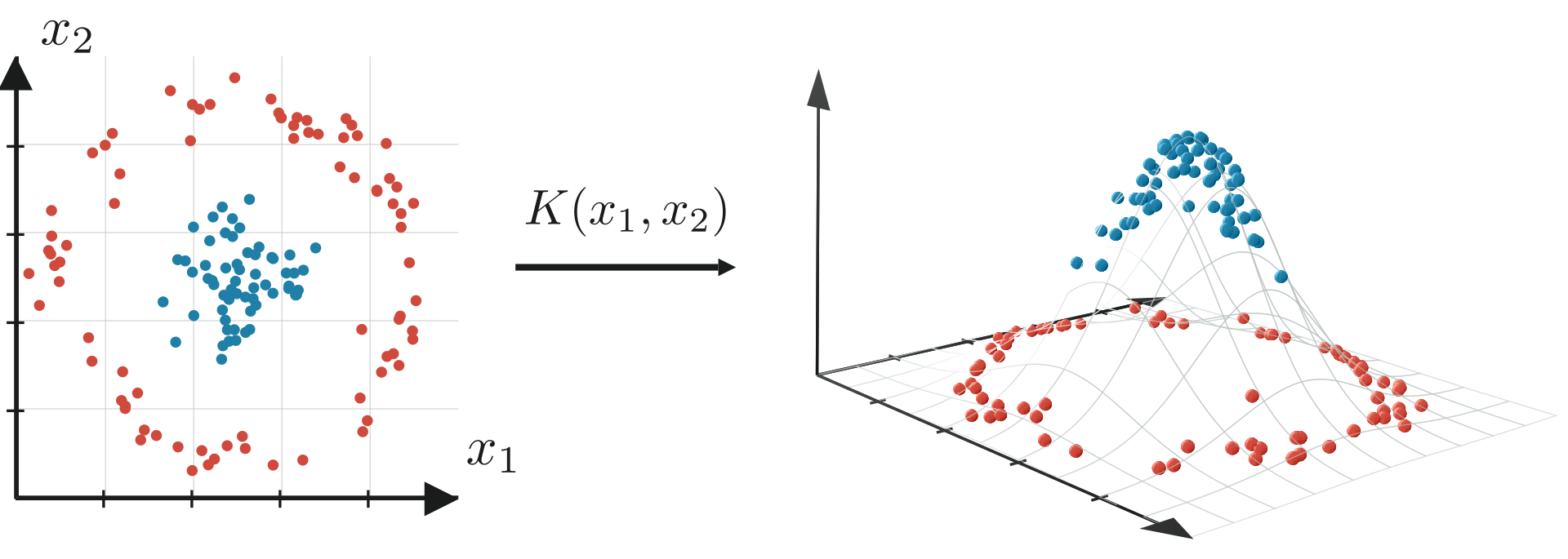
But what if the data isn’t just noisy, but truly not separable by a straight line? Even with slack variables, a linear boundary may still perform poorly if the underlying relationship is non-linear.

Feature Map

The solution is to transform the data into a higher-dimensional feature space where a linear separator does exist. For any dataset, there is always some mapping $\phi(x)$ that makes the data linearly separable in a higher dimension.

$$\phi: \mathbb{R}^n \rightarrow \mathbb{R}^m, \quad m > n$$

For example, we can transform a 1D input $x$ into 2D: $\phi(x) = (x, \; x^2)$. In this new space, a line might separate the data mapped into two-dimensional space where it was otherwise impossible before.

The problem is some feature mappings expand into millions of new features, and others can be infinite-dimensional. Computing all these features is expensive and impractical.

The Kernel “Trick”

When we derived the dual problem for SVMs, notice what appeared:

$$\sum_i \sum_j \lambda_i \lambda_j y_i y_j x_i^T x_j$$

The optimization depends only on the dot product between two data points. So if we transform this data with a feature map, we’d get:

$$\phi(x_i)^T\phi(x_j)$$

Instead of explicitly computing $\phi(x)$, we define a kernel function:

$$K(x_i, x_j) = \phi(x_i)^T\phi(x_j)$$

This lets us work as if we had mapped the data into the higher-dimensional space, without ever computing the coordinates. This is why kernels are sometimes called a trick. It’s a workaround to avoid expensive calculations by performing the dot product in the original low-dimensional space, then using the kernel to find its equivalent feature mapping in the higher-dimensional space.

Polynomial Example

Suppose our inputs are 2-dimensional, and we want to map our features into quadratic space:

$$a = (a_1, a_2), \quad b = (b_1, b_2)$$

A quadratic mapping expands each vector into all degree-2 polynomial terms:

$$\phi(x) = (x_1^2, \; \sqrt{2} x_1 x_2, \; x_2^2)$$

The dot product in this expanded space is:

$$\phi(a)^T\phi(b) = a_1^2 b_1^2 + 2 a_1 a_2 b_1 b_2 + a_2^2 b_2^2$$

This is much more complicated than our original dot product $a^Tb = a_1b_1 + a_2b_2$. And if our original inputs were $n$-dimensional, the expanded quadratic space would have $\tfrac{n^2+n}{2}$ features. It grows quickly!

If you’ve had lots of experience with factoring polynomials, you may notice that:

$$(a^Tb)^2 = (a_1 b_1 + a_2 b_2)^2 = a_1^2 b_1^2 + 2 a_1 a_2 b_1 b_2 + a_2^2 b_2^2$$

which is exactly the same as $\phi(a)^T\phi(b)$! So instead of explicitly computing the feature mapping, we can define a kernel function that automatically computes the same mapping.

General Polynomial Kernel

More generally, the polynomial kernel is:

$$K(a, b) = (a^Tb + c)^d$$

where:

• $c \geq 0$ controls the influence of lower-order terms (usually 1),
• $d$ is the degree of the polynomial expansion.

There are many different kinds of kernel functions out there. But not all functions are kernels.

What Defines a Kernel?

Consider a finite set of $m$ points; let matrix $K$ be defined as:

A function $K$ is a kernel function if and only if its corresponding kernel matrix is:

• Symmetric — a square matrix where it is equal to its own transpose (i.e., $K=K^T$).
• Positive semi-definite — for any input vector $x$, $x^TKx \geq 0$.

This is known as Mercer’s Theorem.

Wrapping Up

Support Vector Machines bring together geometry, optimization, and linear algebra into a beautifully unified model. It’s one of my personal favorites because it’s so intuitive to visualize.

Imagine you’re asked to place the hour hand of an analog clock exactly halfway between the 1 and 5. You would naturally point it at the 3.

• The 1 and 5 are like the support vectors; they’re the closest constraints that determine your choice.
• The other numbers on the clock don’t matter, just as non-support vectors don’t affect the decision boundary.
• The hour hand is the decision boundary itself, positioned to maximize the distance from the critical points on either side.

Just as the 3 is the most balanced position between 1 and 5, the SVM finds the most balanced boundary between two classes. SVMs remain one of the best examples of how theory and intuition meet to produce a model that is both mathematically elegant and practically powerful.