Logistic Regression: Turning Probabilities into Predictions

This post builds off the ideas and notation introuced in the previous two posts:

• How Linear Regression Works (and Why it’s the Foundation of Machine Learning)
• From Lines to Layers: The Linear Perceptron and the Rise of Neural Networks

At their core, logistic regression and other classifiers like the linear perceptron share the same fundamental goal: assign a class to a set of data points. At first glance, they seem almost identical. Both draw a decision boundary to separate points and compute a weighted sum of inputs to make predictions. Where they differ is how they produce those predictions.

The perceptron makes hard, binary decisions: yes or no, 1 or 0. Logistic regression, on the other hand, outputs the probability that a data point belong to a given class. The perceptron updates its weights only when it makes a wrong prediction, while logistic regression updates continuously based on how confident or wrong it was.

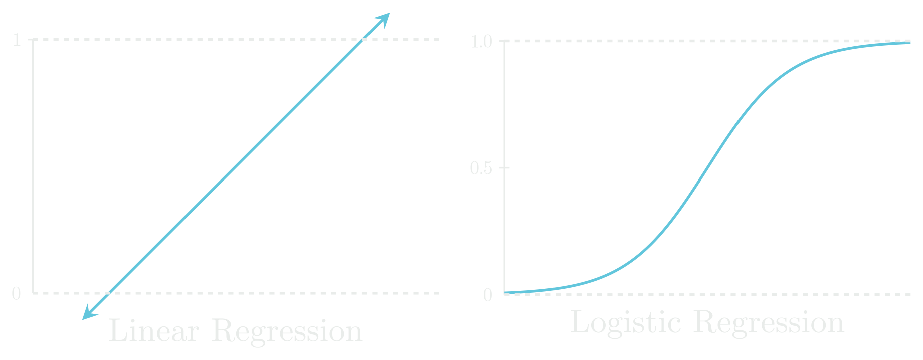
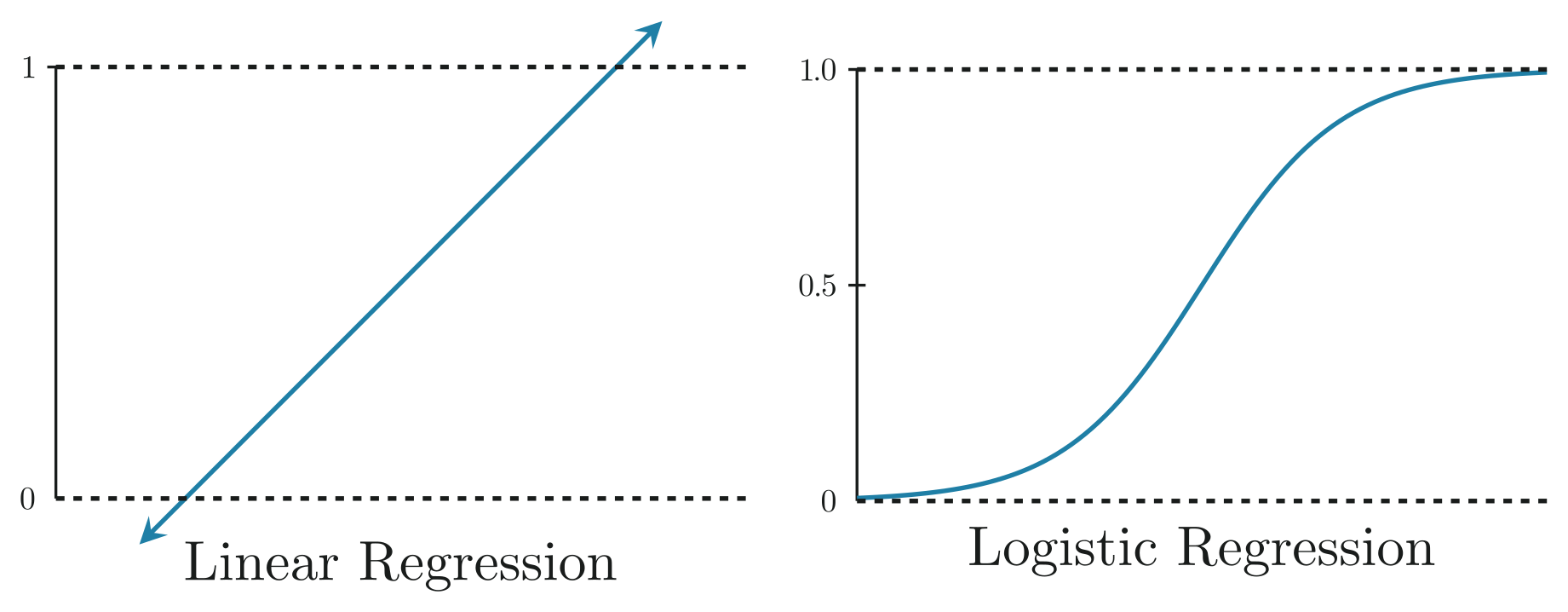
Linear vs Logistic Regression

Unlike linear regression, logistic regression’s output is bounded between 0 to 1, representing the probability that a given set of features belongs to a particular class. To bound the output, we use the sigmoid function:

$$\sigma(z) = \frac{1}{1+e^{-z}}$$

Why Sigmoid?

• Bounded between 0 to 1
• Monotonically Increasing, which means if $x_i < x_j$, then $f(x_i) < f(x_j)$
• Convenient derivative: $\sigma'(x)=\sigma(x)(1-\sigma(x))$, which makes optimization simpler

Turning Output into Decisions

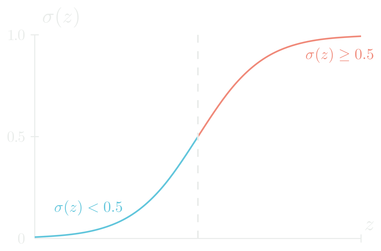
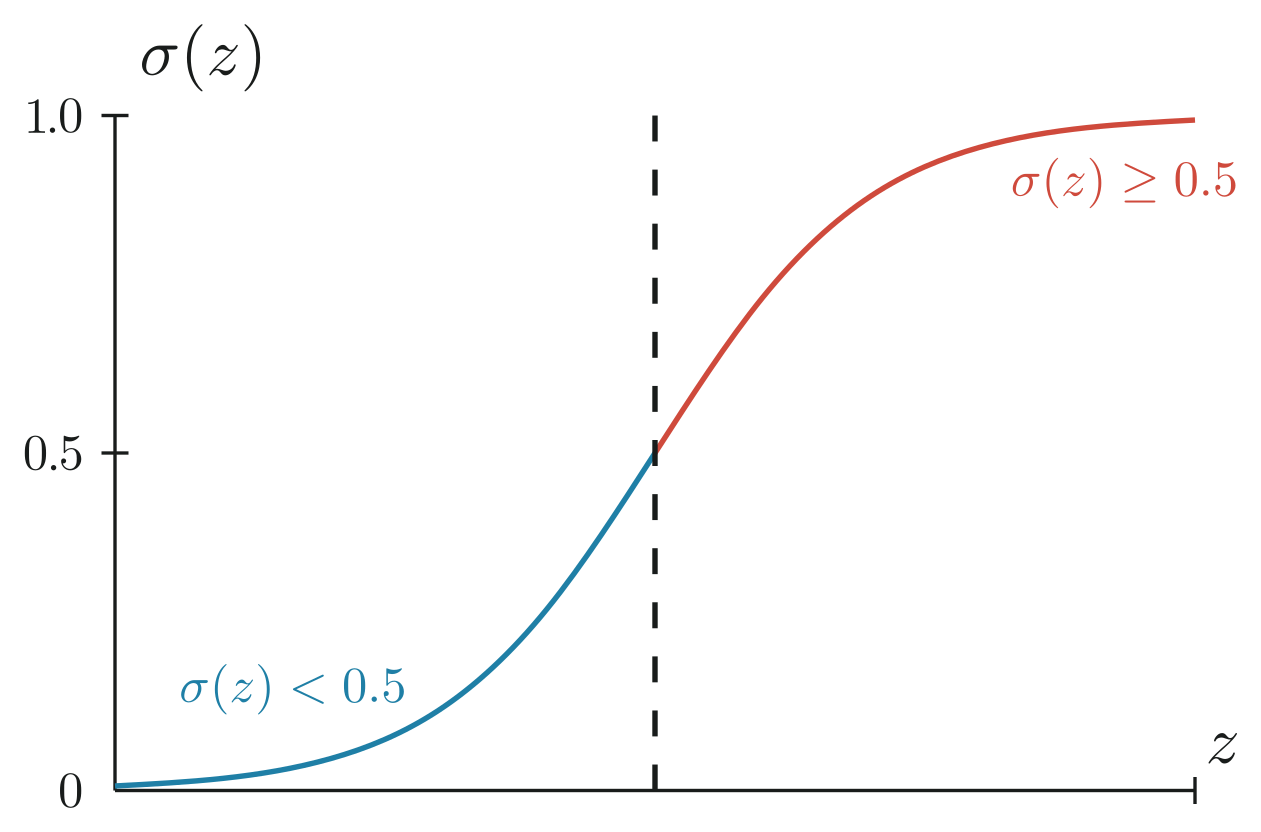
To turn a predicted probability into a class decision, we apply a simple threshold:

$$f(z) = \begin{cases} 1, & \sigma(z) \geq 0.5 \\ 0, & \sigma(z) < 0.5 \end{cases}$$

Here, $z=w^Tx$ is the weighted sum of inputs.

Probability vs. Likelihood

Probability answers the following question:

“Given what I know about the world (my parameters), how likely is a certain event?”

$$P(\text{event} \mid \text{parameters})$$

Imagine you’re shooting arrows at a target. The target’s size, your skill level, wind speed, etc. are all your parameters. If those parameters are fixed, you can calculate the chance that your arrow lands in the bullseye. For example:

• Your shooting pattern follows a certain spread (say, a Gaussian Distribution centered on the bullseye).
• The height of the curve at any point tells you how dense the probability is there i.e., how likely arrows are to land around that point compared to others.
• The actual probability of hitting the bullseye is the area under the curve covering the bullseye region.

If the bullseye covers 10% of the total area under your shooting distribution, then:

$$P(\text{bullseye} \mid \text{parameters}) = 0.10$$

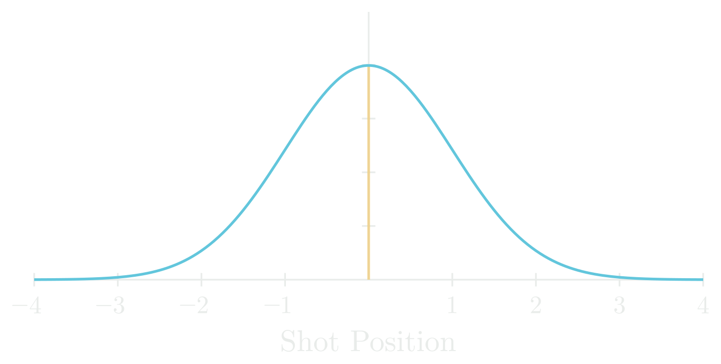
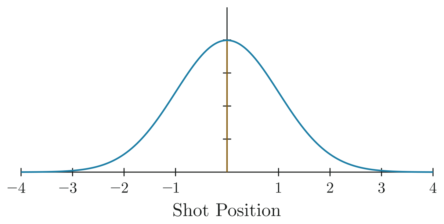
Here, the parameters (spread, aim) are known and the event (whether you hit the bullseye) is unknown.

Likelihood

Likelihood asks the opposite question:

“Given that I already observed an event, which parameter values make that observation most probable?”

$$L(\text{parameters} \mid \text{event}) = P(\text{event} \mid \text{parameters})$$

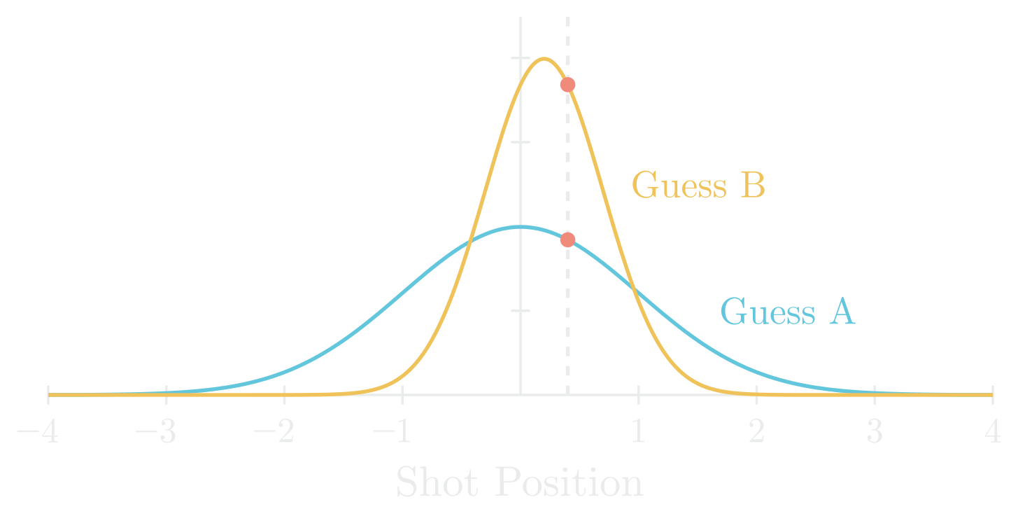
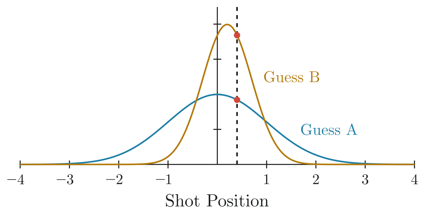
Now imagine that the arrow has already hit the target. The question then becomes: Which shooting pattern would make this hit seem most natural?

For example:

• Guess A: Your shots usually spread widely, hitting this exact spot would be rare.
• Guess B: Your shots cluster tightly around this spot, hitting here would be very likely.

Since Guess B’s distribution is more dense where the arrow landed than Guess A’s, Guess B is more consistent with the observation.

If you still aren’t sure of the difference between probability and likelihood, I highly recommend watching this short video:

From Statistics to Machine Learning

In logistic regression:

• Parameters — The model’s weights $w$
• Observations — Feature matrix $X$ and labels $y$. Each $x^{(i)}$ has $n$ features for $m$ examples.

$$X = \begin{bmatrix} | & | & | & |\\ x^{(1)} & x^{(2)} & \dots & x^{(m)} \\| & | & | & | \end{bmatrix}^T \quad y = \begin{bmatrix} y^{(1)} \\ y^{(2)} \\ \vdots \\ y^{(m)} \end{bmatrix}$$

Why is $X$ a matrix?

When you first learn about logistic regression or cross-entropy loss, it’s tempting to work through everything with just a single example. That makes the math easier to see, but it’s not how these algorithms are actually used in practice. In reality, we almost always deal with many examples at once. Libraries like PyTorch or TensorFlow all expect you to feed in batches of examples at a time. They rely on vectorized matrix operations under the hood because it’s massively faster than looping through one example at a time. Once you’re comfortable thinking in terms of batches and matrix operations, moving into practical ML work feels much more natural.

If we assume each example is independent of one another, then the probability of assigning each label $y^{(i)}$ to feature $x^{(i)}$ under weights $w$ is the product of their individual probabilities.

$$L(w \mid X, y) = P(y \mid X ; w) = \prod_{i=1}^m P(y^{(i)} \mid x^{(i)} ; w)$$

Since we are dealing with binary classification, the probability of an example being in the positive class is the same as it not being the negative class:

$$P(y^{(i)} = 1 \mid x^{(i)} ; w) = 1 - P(y^{(i)} = 0 \mid x^{(i)} ; w)$$

To express both cases in a single formula, we write:

$$P(y^{(i)} \mid x^{(i)} ; w) = (\hat{y}^{(i)})^{y^{(i)}} (1 - \hat{y}^{(i)})^{1 - y^{(i)}}$$

where $\hat{y}^{(i)} = \sigma (w^Tx^{(i)})$ is the predicted probability from our sigmoid activation function. This is just a clever algebra trick to succinctly merge the two cases into a single expression.

• If $y^{(i)} = 1: P(y^{(i)} \mid x^{(i)} ; w) = \hat{y}^{(i)}$
• If $y^{(i)} = 0: P(y^{(i)} \mid x^{(i)} ; w) = 1 - \hat{y}^{(i)}$

Maximizing Likelihood

In machine learning, our goal is to choose weights that maximize the likelihood of our observed data. This approach is called the Maximum Likelihood Estimator (MLE). The MLE finds the “optimal” weights $w^*$ that make the observed data most probable under our model.

$$w^* = \underset{w}{\arg\max} \; L(w \mid X, y) = \underset{w}{\arg\max} \; \prod_{i=1}^m P(y^{(i)} \mid x^{(i)} ; w)$$

However, computing this directly is challenging. Taking the product of many probabilities can cause numerical underflow, where values become too small for the computer to represent accurately. Additionally, differentiating a product of many terms is computationally expensive.

Log-Likelihood

To address these issues, we can take advantage of the logarithmic property:

$$\log(ab)=\log(a)+\log(b)$$

The core idea behind this is that we’re replacing a difficult and expensive product with an easier to handle sum. Applying this to our likelihood gives us:

$$\begin{align*} \log L(w \mid X, y) &= \log \prod_{i=1}^m P(y^{(i)} \mid x^{(i)} ; w)\\ &= \sum_{i=1}^m \log P(y^{(i)} \mid x^{(i)} ; w)\\ &= \sum_{i=1}^m \left[ y^{(i)} \log \hat{y}^{(i)} + (1 - y^{(i)}) \log (1 - \hat{y}^{(i)}) \right]\\ \end{align*}$$

Why can we take the log of the likelihood?

Because the logarithm function is a monotonic function and is always increasing in one direction. We are essentially just scaling the output values (y-axis) of the graph while the peaks and valleys location (x-axis) stay at the same value. Thus, the weights that maximize the likelihood are the same as the ones that maximize log-likelihood.

Binary Cross-Entropy (a.k.a Negative Log-Likelihood)

Binary Cross-entropy (BCE) is simply negative log-likelihood for binary classification. It measures how well the predicted probabilities match the true labels:

$$BCE(w) = - \frac{1}{m} \sum_{i=1}^m \left[ y^{(i)} \log \hat{y}^{(i)} + (1 - y^{(i)}) \log (1 - \hat{y}^{(i)}) \right]$$

• If $y^{(i)} = 1$: the second term is zero, and the loss penalizes a low predicted probability for the positive class.
• If $y^{(i)} = 0$: the first term is zero, and the loss penalizes a high predicted probability for the positive class.

Note: we usually scale the loss by the number of examples $m$. In batch training, we may have different batch sizes, and want our loss to be at a consistent scale across batches.

Examples

$$BCE_i = - \left[ \log 0.7 + \log 0.9 + \log (1 - 0.2) + \log 0.8 + \log (1 - 0.3) \right] \approx 1.265$$ $$BCE_j = - \left[ \log 0.6 + \log 0.3 + \log (1 - 0.5) + \log 0.5 + \log (1 - 0.8) \right] \approx 4.711$$

A lower BCE means better predictions. Confident and correct predictions yield small loss values, while confident but wrong predictions yield large losses.

Finding $w^*$

Most optimization algorithms are designed to minimize functions rather than maximize them. Instead of maximizing log-likelihood, we minimize the negative log-likelihood (BCE):

$$w^* = \underset{w}{\arg\min} \; BCE(w)$$

Since we cannot solve for $w^*$ analytically, we must use an iterative optimization algorithm like gradient descent. The gradient of BCE with respect to our weights is:

$$\nabla_w \; J(w) = \frac{1}{m} X^T \left(\hat{y}^{(i)} - y^{(i)} \right)$$

Derivation

We then iteratively update our weights:

$$w_{t+1} = w_t - \alpha \cdot \nabla_w J(w)$$

where $\alpha$ is the learning rate. Over time, this process finds the $w$ that minimizes BCE, and equivalently, maximizes the likelihood of the observed data.

Multiclass Classification

In binary classification, our model outputs a single probability for the positive class. For example, given an input $x^{(i)}$, we might predict $\hat{y}^{(i)} = 0.85$, meaning we believe there’s an 85% chance it belongs to class 1 (and a 15% chance it belongs to class 0).

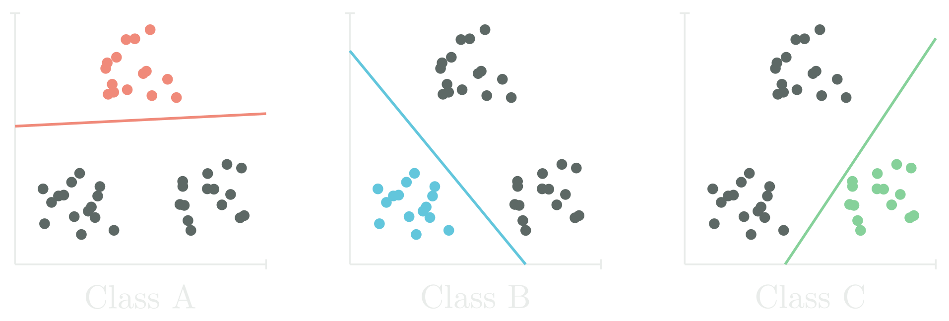
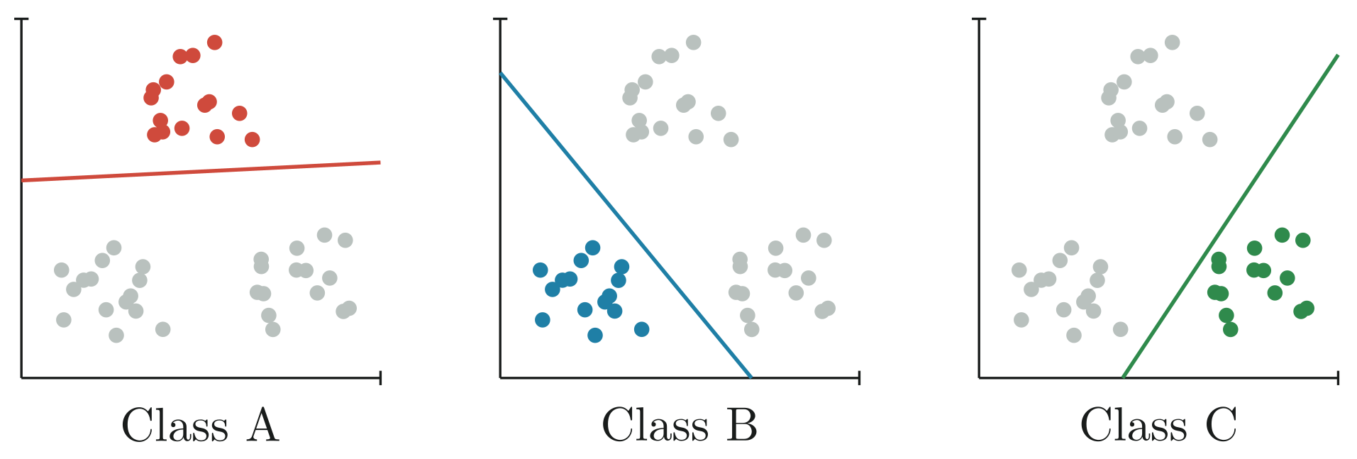
When moving to multiclass classification, instead of just two outcomes, we have $K$ possible classes, and our model must output a full probability distribution over these classes. This means:

• Each probability must be between 0 and 1.
• All $K$ probabilities must sum to 1.

Representing Model Parameters

To seperate $K$ classes, we need $K$ decision boundaries. Each decision boundary has its own weight vector $w_k$. If each example $x^{(i)}$ has $n$ features, then the weights of our model becomes a matrix:

$$W = \begin{bmatrix} | & | & | & |\\ w_1 & w_2 & \dots & w_K\\| & | & | & | \end{bmatrix} \in \mathbb{R}^{n \times K}$$

Logits

For binary classification, the logit is $z = w^Tx$. In multiclass classification, we compute one logit per class:

$$z^{(i)}_k = w_k^Tx^{(i)}$$

Instead of computing them one-by-one, we can get all logits at once:

$$Z = XW$$

Softmax Activation

To turn logits into valid probabilities, we use the softmax activation function:

$$\hat{y}^{(i)}_k = \text{softmax}\left( z^{(i)}_k \right) = \frac{e^{z^{(i)}_k}}{\sum_{j=1}^K e^{z^{(i)}_j}}$$

Softmax guaruntees that all probabilities are positive and sum to 1. When $K=2$ softmax reduces to the sigmoid function. Try it out for yourself!

We can store all predictions for all examples in:

$$\hat{Y} = \text{softmax}(Z)$$

Representing True Labels

We use one-hot encoding so that each label is a vector indicating the correct class:

• $y^{(i)}_k = 1$ if example $i$ belongs to class $k$
• $y^{(i)}_k = 0$ otherwise

Likelihood Function

In multiclass classification, we care only about the probability our model assigns to the correct class for each example. For a single example $i$, this is written as:

$$P(y^{(i)} \mid x^{(i)}; W) = \prod_{k=1}^K \left( \hat{y}^{(i)}_k \right)^{y^{(i)}_k}$$

Why this works:

• The label vector $y^{(i)}$ is one-hot encoded, so only the correct class has $y^{(i)}_k = 1$.
• All incorrect classes have $y^{(i)}_k = 0$, which means their probabilities are raised to the power of zero and disappear from the product.
• What’s left is just the predicted probability of the true class.

Over all $m$ examples, the total likelihood becomes:

$$L(W \mid X, Y) = \prod_{i=1}^m \prod_{k=1}^K \left( \hat{y}^{(i)}_k \right)^{y^{(i)}_k}$$

Log-Likelihood and Cross-Entropy

Just like before, we turn our products into sums by taking the log of the likelihood function:

$$\log L(W \mid X, Y) = \sum_{i=1}^m \sum_{k=1}^K y^{(i)}_k \log \hat{y}^{(i)}_k$$

Our goal is to find the weights $W^*$ that maximize this log-likelihood. Equivalently, we can minimize the negative log-likelihood (i.e., cross-entropy loss):

$$W^* = \underset{W}{\arg\min} \; \text{CE}(W) = - \frac{1}{m} \sum_{i=1}^m \sum_{k=1}^K y^{(i)}_k \log \hat{y}^{(i)}_k$$

Optimization

There’s no closed-form solution for $W^*$, so we use gradient descent again to find the optimal weights. The gradient of CE with respect to the weights is nearly identical to the binary case:

$$\nabla_W J(W) = \frac{1}{m} X^T(\hat{Y} - Y)$$

This tells us exactly how to adjust each weight to reduce the error.

Wrapping Up

At its heart, logistic regression, binary or multiclass, is about answering:

“Given the data I’ve seen, which class is most likely?”

Binary classification is a simple yes/no decision. Multiclass extends the idea: we compute a score for each class, transform those scores into probabilities with softmax, and pick the highest.

This is the third supervised learning algorithm we have covered, and you should start to notice a pattern with how these models learn from data.

1. Define what “good” means (probability of the correct class).
2. Measure how bad we did (loss function).
3. Adjust the weights to do better next time (gradient descent).

The cycle repeats: predict $\rightarrow$ measure $\rightarrow$ improve.