The Math Behind Machine Learning
If terms like gradients, dot products, or partial derivatives feel a little rusty, this post walks through the key math behind machine learning: linear algebra, calculus, and probability, without diving too deep.
Machine learning is about teaching computers to find patterns in data. While many frameworks let you build models without diving into the math, understanding the underlying concepts, especially in linear algebra and calculus, can give you a much deeper intuition for how these systems work and why they behave the way they do.
In this post, I’ll walk through the most important topics in linear algebra and calculus that you’ll see across machine learning models, from linear regression to neural networks.
Linear Algebra in Machine Learning
Linear algebra is the language of machine learning. We can represent our data using vectors and matrices and many machine learning algorithms are simply manipulating our data through matrix operations.
1. Vectors
A vector is just an ordered list of numbers, often used to represent a point in space, a direction, or a collection of features for a data point. In machine learning, vectors commonly represent inputs like measurements or attributes.
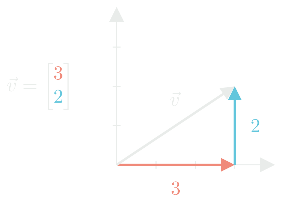
The illustration below shows how a vector can be broken down into its component vectors, with each component having a length (or magnitude) along an axis. These components stack together, starting from the origin and extending through each axis direction.
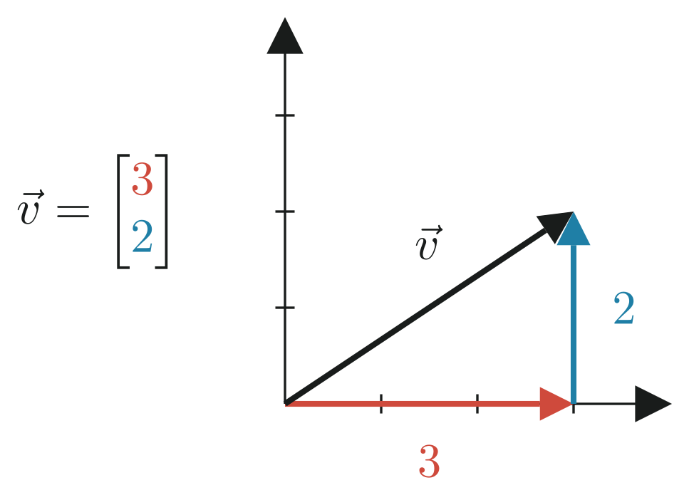
This idea is easy to visualize in two or three dimensions. But as we move into higher-dimensional spaces, where each feature becomes its own axis, visualizing vectors becomes impossible. That’s normal. Just keep in mind that the same principles apply, even if we can’t “see” them.
Vector Operations
-
Addition & Subtraction
This represents combining two vectors element by element. You can think of it as adding two measurements together.
-
Scalar Multiplication
This scales each component of the vector. It’s like turning up the volume of all features equally.
-
Dot Product
The dot product measures how similar two vectors are in direction. A higher value means they point in a more similar direction.
-
Norm (Vector Magnitude)
The norm is the length of the vector, calculated using the Pythagorean theorem. It’s often used to measure the size or distance of a data point from the origin.
2. Matrices
A matrix is just a table of numbers. If you’ve ever used Excel or Google Sheets, you’ve already worked with something like a matrix. In machine learning, we use matrices to represent entire datasets. Each row is usually a data point, and each column is a feature or attribute.
| Height (in.) | Weight (lb.) | Age |
|---|---|---|
| 70 | 160 | 28 |
| 65 | 130 | 22 |
| 72 | 180 | 31 |
We can write this table as a matrix like this:
You may have noticed that a matrix is essentially a group of vectors stacked on top of each other (as rows) or arranged side by side (as columns). In machine learning, we usually treat each row of a matrix as a separate data point, and each column as a different feature.
So if you have a dataset with 100 examples and 3 features (like height, weight, and age), you can represent it as a matrix with 100 rows and 3 columns
A Quick Note on Tensors
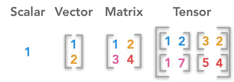
A tensor is a general way to describe a container of data. Just as a vector is a one-dimensional list of numbers, and a matrix is a two-dimensional grid, a tensor can have any number of dimensions. So really, tensors are the umbrella term to describe scalars, vectors, and matrices.
Tensors have three main properties:
-
Rank — This just means how many dimensions the tensor has. A scalar has rank 0, a vector has rank 1, a matrix has rank 2, and so on. A rank-3 tensor might describe something like an RGB image, and rank-4 or higher is common in deep learning.
-
Shape — The shape tells you the size of the tensor along each dimension. For instance, the shape of the previous matrix example has shape . A vector with 5 elements has shape (the trailing comma tells us it’s a 1D shape, not just a plain number). A scalar, being just a single number, has shape . You may also see the shape of a matrix defined as , which defines the set of values the matrix can take (set of real numbers in this case), and then the number of rows, columns, … ( and ).
-
Data Type — Tensors usually store numbers (like integers or floats), but they can hold other types too, like strings or booleans.
Tensors with more than two dimensions are useful for representing more complex data. For example, you can represent a video as a rank-4 tensor with shape , where the last dimension corresponds to color channels (red, green, blue).
While we won’t go too deep into high-rank tensors here, it’s helpful to know that scalars, vectors, and matrices are just special cases of tensors. The concept of shape becomes especially important when doing operations on tensors. If the shapes don’t match in the right way, the operation won’t work.
Matrix Operations
-
Matrix Addition & Subtraction
Note: matrices must be the same shape
-
Matrix Multiplication
Unlike addition, matrix multiplication is not element-wise. Instead, it involves combining rows from the first matrix with the columns from the second.
Note: the number of columns in the first matrix must equal the number of rows in the second. The resulting matrix will have the number of rows in the first matrix and the number of columns in the second.
-
Transpose
This flips the matrix, turning rows into columns. It’s often used when aligning the data for matrix operations.
-
Identity Matrix
Like the number 1, any matrix multiplied by the identity matrix stays the same.
-
Inverse Matrix
The inverse of a matrix is like the reciprocal of a number (e.g., the reciprocal of is because ). Similarly, the inverse of matrix is the matrix that satisfies .
Matrix inverses are used in certain algorithms, but in practice, we avoid calculating directly because it can be computationally expensive and unstable. You can learn more about how to calculate the inverse of a matrix here.
3. Linear Transformations
Many machine learning models are built on linear transformations, which are essentially functions that scale, rotate, or project data using matrix multiplication. So far, we’ve looked at matrices as just tables of numbers, but they actually describe transformations of space. Think of a matrix not just as a data container, but as a function that reshapes or moves vectors.
A great tool to help visualize these transformations can be found here. The 3Blue1Brown video below is also a great reference to gain a better understanding of how this works.
Calculus in Machine Learning
Calculus can feel intimidating, especially if it’s been a while since you last saw it. But I can assure you that as someone who was never the biggest fan of calculus, a basic understanding of its key concepts and rules is more than enough for most applications. Still, there’s great value in understanding what’s happening behind the scenes. I’ll walk through the core ideas at a high level, without diving into any math.
1. Derivatives
A derivative tells us how a function changes as its input changes (i.e., slope or rate of change). If a function’s input increases slightly, the derivative tells us how much the output will increase (or decrease) as a result. In machine learning, we use derivatives to understand how the loss function, which measures how wrong our model is, changes as we tweak the model’s parameters (like weights in a neural network).
2. Gradients
A gradient is a generalization of the derivative for functions with multiple inputs. It’s a vector that contains all the partial derivatives with respect to each input. Each partial derivative tells us how much the output would change if we nudged just one input a little, keeping the others fixed.
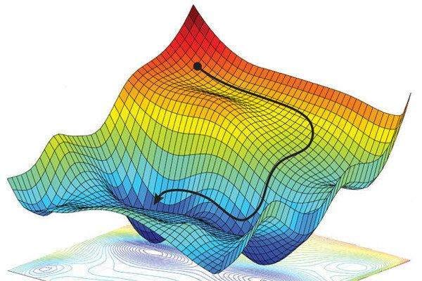
In machine learning, the gradient points in the direction of steepest increase of the loss function. To improve the model, we move in the opposite direction, called the negative gradient, which reduces the loss. This process is called gradient descent, and it’s one of the core techniques behind training models.
3. Chain Rule
The chain rule lets us compute the derivative of functions that are made up of other functions. For instance, when one function’s output is the input to another. This is especially important in neural networks, where each layer passes its output to the next. Using the chain rule, we can “chain together” derivatives from the final output all the way back to the first layer. This is the key idea behind backpropagation, the algorithm used to train deep learning models.
What’s next?
If this post refreshed a few concepts for you, great. Understanding the math behind machine learning doesn’t mean you need to be able to do matrix multiplication or calculate partial derivatives. Thanks to libraries like TensorFlow, PyTorch, and Keras, you rarely need to do any math by hand. But having an intuition for concepts like vectors, matrices, gradients, and derivatives can help you see how these models work under the hood and understand why they behave the way they do.
I believe the best way to learn is through trial and error. In future posts, I’ll break down how these ideas apply directly to machine learning, and how to build your own models and algorithms.