How Linear Regression Works (and Why it's the Foundation of Machine Learning)
What linear regression is, how it makes predictions, and how it learns from data. This one model introduces feature vectors, model parameters, loss functions, and gradient descent.
If you’re just starting to explore machine learning, it can be tempting to jump straight into complex models like neural networks or decision trees. But beneath all of that complexity is a surprisingly simple and powerful idea: linear regression.
Linear Regression is a type of supervised learning algorithm, which means in our dataset we know what the expected result should be, and we can compare the model’s predictions with the expected result. In the case of linear regression, the expected result is some number. The goal of linear regression is to find some relationship between the inputs (features) and the output (label).
For example, let’s say we want to predict the price of a house given its size. We can collect housing data and plot a bunch of points on a graph of how the size of a house affects its price. With enough data, we can start to draw a line of best fit through those data points in order to predict future house prices.
| Size () | Price ($) |
|---|---|
| 1,300 | 360,000 |
| 1,800 | 540,000 |
| 2,200 | 770,000 |
| 2,400 | 864,000 |
| 3,000 | 990,000 |
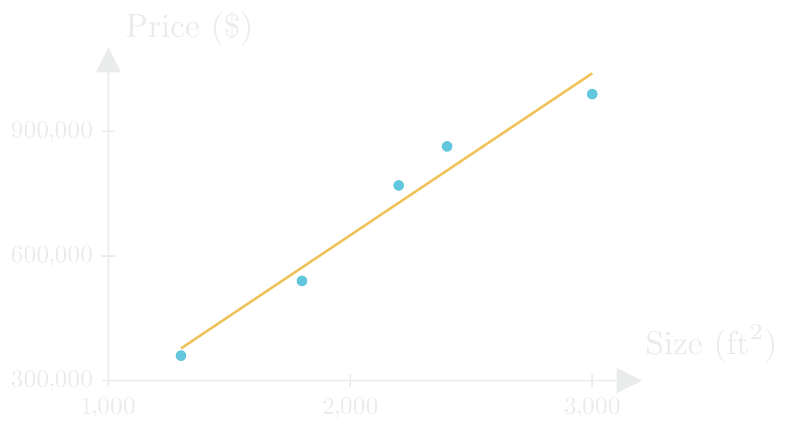
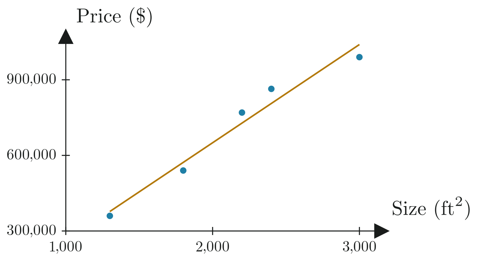
This scales beyond just one input. With multiple features (number of rooms, location, etc.), instead of fitting a line in two dimensions, we’re fitting a plane or hyperplane in higher dimensions.
The Linear Model
You may recall from your algebra class that the equation for a straight line is . This formula tells us that for every unit increase in , the output increases by . In machine learning, we use a similar idea, but instead of just one input, we often have many. Each input is a feature, and we want to learn how much each one contributes to the final prediction.
From One Feature to Many
To generalize the line equation to work with multiple features, we turn our input into a vector:
And assign each feature its own weight:
Then, the prediction is:
This is our linear model, where:
- is the predicted value
- is the input vector of features
- is the weight vector
- is the bias (same as the intercept in )
Each weight tells us how strongly that feature influences the prediction. The model combines all the weighted inputs and adds the bias to produce the output.
From One Example to Many
So far, we’ve described a single prediction for one input. But machine learning models are trained on many examples at once. If we have training examples, each with features, we can stack all our input vectors into a matrix:
This matrix is called the design matrix, where each row is an example and each column is a feature. This is pretty useful because we can make predictions for all examples with just one matrix operation:
A Note on Bias Handling
Some implementations absorb the bias term into the weight vector by adding an extra feature that is always 1:
Then the prediction becomes:
This form simplifies the math. In the future you may see me use this notation but for this post we’ll keep and separate for clarity.
Measuring Error
The difference between the true value and the predicted value is called the residual:
This represents how far off the model’s prediction was for example . If the residual is large, the prediction was poor. If it’s close to zero, the prediction was accurate.
To keep track of individual examples, we use a subscript to indicate which prediction we’re referring to.
Loss Functions
Once our model is making predictions, we need a way to measure how well it’s performing across all data points. This is where a loss function comes in. Just like choosing the right model for a task, picking the right loss function can make the difference between a model making accurate or misleading predictions. There are many different types of loss functions, but the most common one used in linear regression is Mean Squared Error (MSE):
Why do we square the residuals?
Residuals can be either positive or negative. If we simply summed them, those positive and negative errors could cancel each other out, making it seem like the model is performing better than it really is.
By squaring each residual, we ensure all errors are positive and that larger mistakes are penalized more heavily than smaller ones. This gives us a more accurate picture of the model’s overall performance.
Limitations
Like I mentioned in my introductory post, machine learning is a set of tools, and knowing what tool to use in certain situations is just as important as understanding how these models work. When we are using linear regression, we are making a few assumptions about our dataset in order to make accurate predictions.
1. Linearity
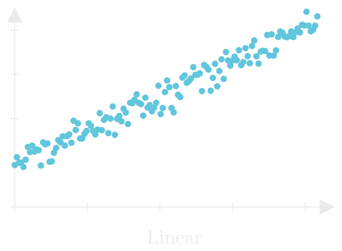
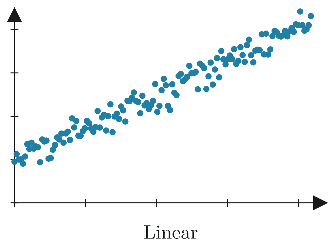
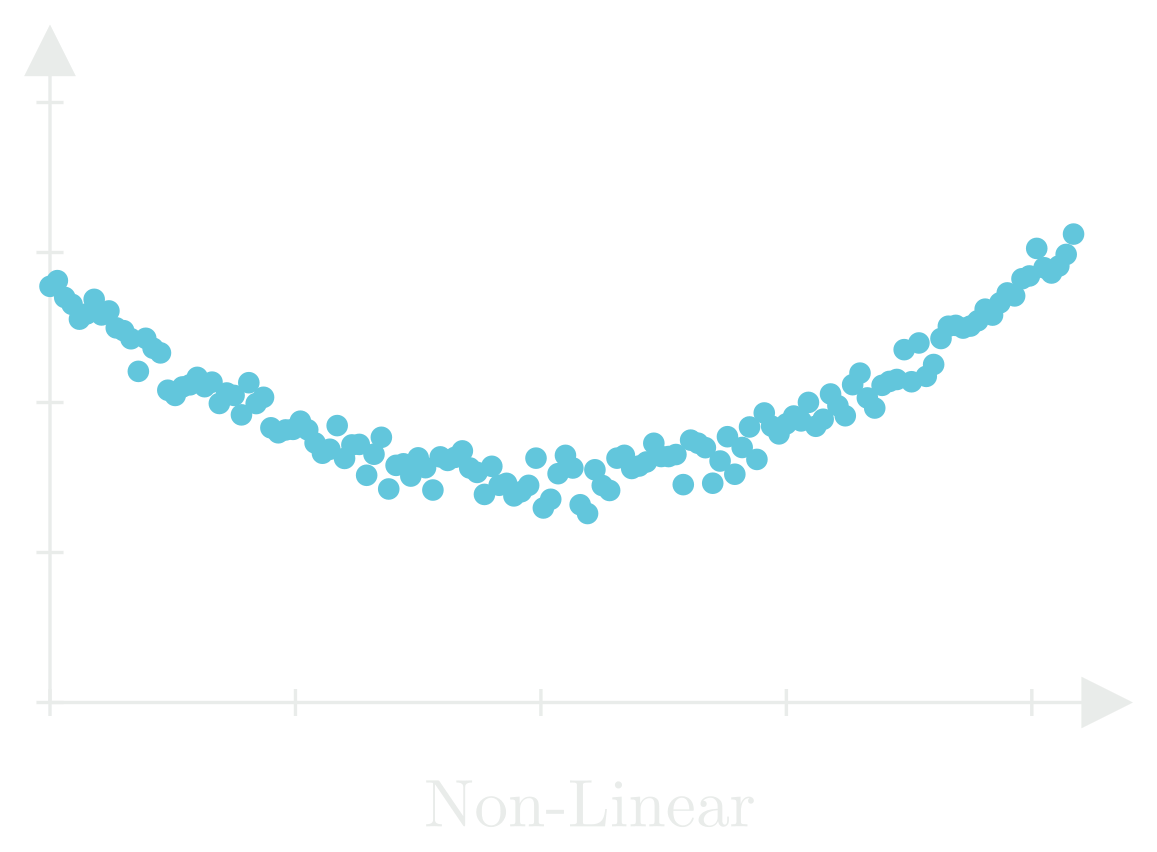
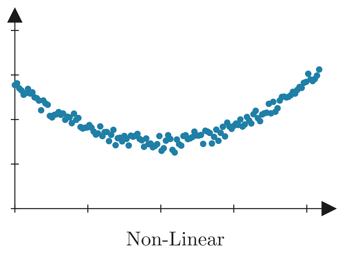
Our first assumption is that there is a linear relationship between our input features and the expected outputs. There is a linear relationship between the size of a house, and its price (i.e., the bigger the house, the higher the price). For many real-world problems, this is usually not the case. If the data forms a curve, a cluster, or changes direction, a linear model won’t capture those patterns well, no matter how much data you give it.
This is where more advanced models like neural networks come in. They can handle non-linear patterns by transforming the input space or using more flexible functions. Still, starting with a linear model is a good baseline.
2. Independent Residuals
Another assumption we are making is that the residuals are independent of one another. This means that the error for one data point shouldn’t affect or predict the error of another. This is especially important in sequential data (like time-series), where the data points are correlated with each other.
3. Identically & Normally Distributed
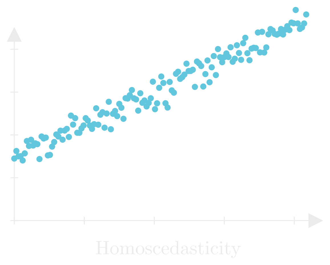
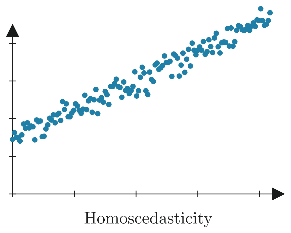
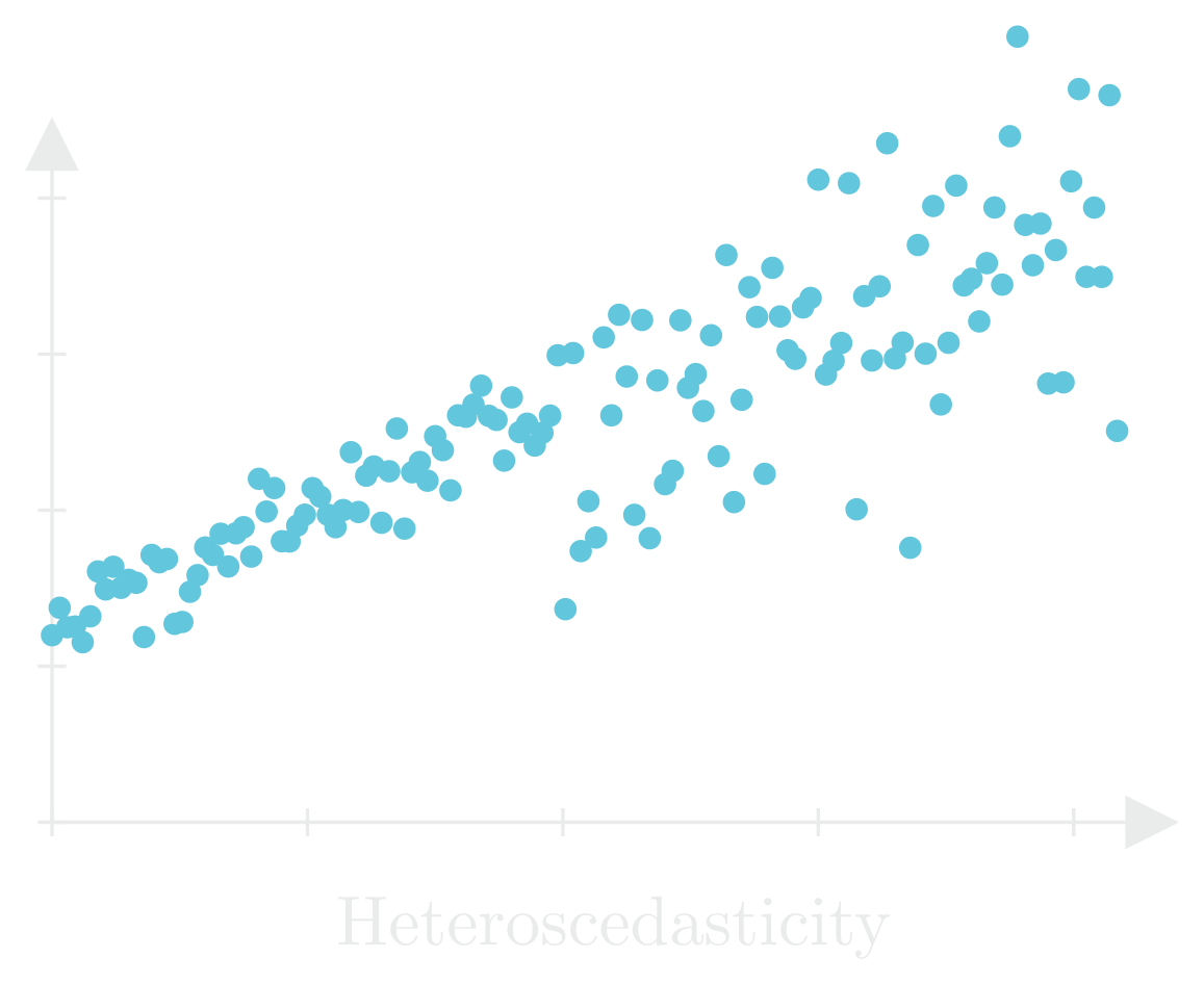
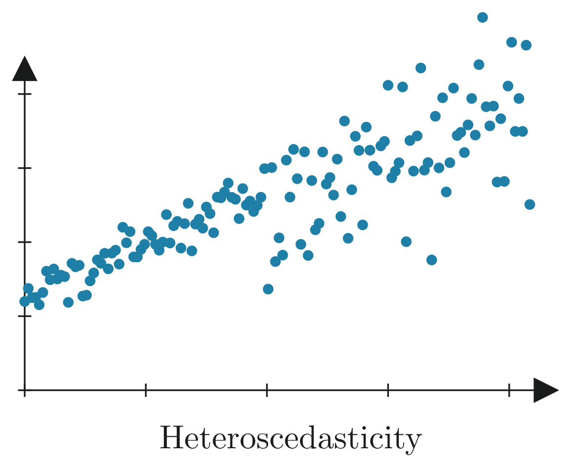
The last assumption we are making is that the residuals follow the same, normal distribution. This means that there should be a constant variance across all data points. If the residuals start to fan out or shrink together, it’s called heteroscedasticity, and will negatively affect the accuracy of the model.
Training the Model
Training simply means finding the best weights that allow the model to make accurate predictions on our data. Now that we can measure our model’s performance via Mean Squared Error, we want to minimize this function in order to achieve the lowest possible error. The model starts off with random weights. At first, it makes bad predictions. Our goal is to adjust the weights so that the model makes better predictions (i.e., the error decreases). This is where gradient descent comes in.
Gradient Descent
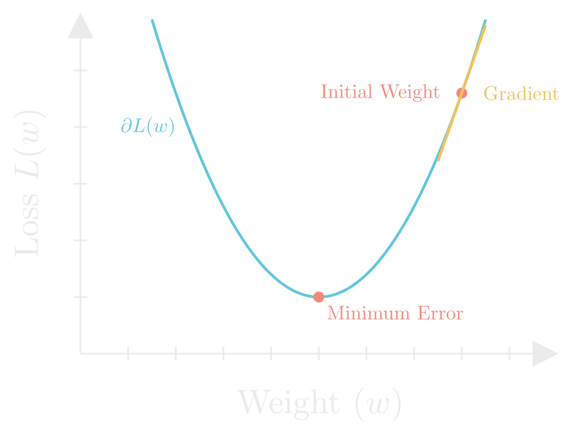
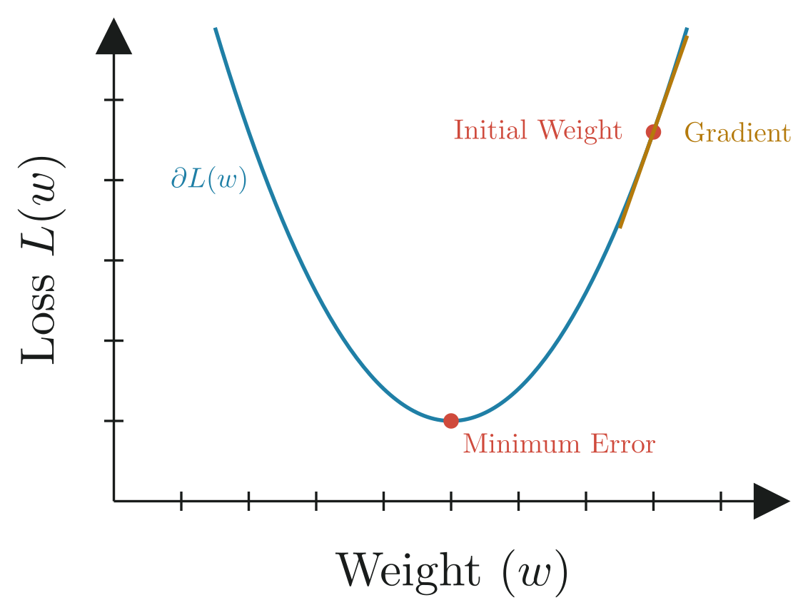
Gradient Descent is an optimization algorithm, which is a method that iteratively adjusts the weights in order to reduce the error of a loss function. You can think of gradient descent as slowly traversing down a foggy mountain. You can’t see the entire landscape, but you can see the slope beneath you and can take small steps downhill, eventually reaching flat ground.
How It Works
- Initialize weights randomly.
- Make predictions using those weights.
- Calculate the loss, which tells us how far off our predictions are.
- Compute the gradient of the loss function with respect to the weights. This tells us the direction and rate of change of the loss.
- Update the weights slightly in the direction that reduces the loss (negative gradient).
- Repeat this process many times until the loss is minimized.
Computing the Gradient
If you haven’t brushed up on calculus recently, you might find it helpful to read my post on the math used in machine learning.
To update our weights using gradient descent, we need to compute the gradient of the loss function with respect to the weight vector. This tells us how changing each weight will affect the model’s error.
We’ll assume:
- We have a dataset with examples
- Each example has features
- is the weight vector
- is the bias term
- is the predicted output
- is the actual label
- is our loss function, Mean Squared Error (MSE):
Taking the Derivative
First, we compute the gradient with respect to :
We also compute the gradient of the loss with respect to :
Updating Our Weights
Now we can update our weights:
Where:
- is the vector of weights we’re updating
- is the current iteration step
- is the learning rate, which controls how large each update step is
- is the loss function we’re trying to minimize
By plugging the computed gradient into this update rule, the model takes a small step in the direction that reduces the error. Repeating this process over many iterations allows the model to “learn” by gradually improving its predictions. This is the core idea behind how most machine learning models are trained.
Implementation
So far, we’ve gone over how linear regression works under the hood, now let’s implement a simple training routine.
from sklearn.linear_model import LinearRegression
from sklearn.model_selection import train_test_split
from sklearn.metrics import mean_squared_error
from matplotlib.pyplot import plt

# Assume X is your feature matrix and y is your target vector

# Split data into training and testing sets
X_train, X_test, y_train, y_test = train_test_split(X, y, test_size=0.2, random_state=42)

# Create the model
model = LinearRegression()

# Train the model
model.fit(X_train, y_train)

# Make predictions
y_pred = model.predict(X_test)

# Evaluate performance
mse = mean_squared_error(y_test, y_pred)
pprint(f"Mean Squared Error: {mse:.2f}")
print("Weights (slope):", model.coef_)
print("Bias (intercept):", model.intercept_)

# Visualization
plt.scatter(X, y, color='blue')
plt.plot(X, model.predict(X), color='red')
plt.show()
What Just Happened?
model.fit()ran the training loop internally, it handled all the gradient computations and updated the weights for you. Neat!model.coef_gives you the learned weights.model.intercept_gives you the bias term.
If you’ve been following along, this simple coding example should make a lot more sense.
Wrapping Up
That was a lot, but hopefully now linear regression doesn’t feel like a mystery. It’s just a model that tries to draw the best line (or hyperplane) through your data by adjusting weights to reduce error. We looked at how it works from both a math and code perspective, and hopefully things are starting to make a little more sense now.
Even though it’s one of the simplest models in machine learning, it’s also one of the most important. A lot of more advanced techniques build off these same core ideas: predictions, loss functions, gradients, and optimization. If you understand this, you’re off to a great start.